Colocalization And Association¶

VIPP supports pixel, ROI-masked, object-restricted, and label-association workflows.

Choose An Example¶

New in 0.15.0a5: The combined example is now two focused workflows under Colocalization & Association in Open example…:

RACC Colocalization shows whole-image and ROI-masked RACC. Both nodes retain Manual thresholds of Ch1 43,970.51 and Ch2 48,073.03; Binary Threshold selects the red-channel ROI at 30,000. Inspect the Magma index images, then change Theta to explore the distance penalty. The notes include the method's full name and paper.
Colocalization, Overlap & Object Counts shows whole-image and ROI-masked overlays and Pearson/Manders metrics, using Costes auto. Its separate Colocalization Mask → Remove Small Objects → Label Connected Components → Measure Objects branch matches the unmasked white overlap. Cleanup keeps face-connected 3D regions of at least 20 voxels. Select Measure Objects to see one row per retained region; lower the minimum size to 1 voxel and recalculate to include the small regions too.

The counting branch is not restricted by the ROI. These settings are tailored to the synthetic sample, not defaults for other images. Reopen the examples from the catalogue for these changes; previously saved workflows are unchanged.

0.13 and later colocalization results can differ from 0.12

VIPP 0.13 and later retain finite native channel intensities rather than jointly scaling/clipping both channels to 0–255. Thresholds and intensity sums now use native units, and the Costes, Pearson, and Manders definitions were revised toward Fiji Coloc 2 3.1.0 semantics. Preserve older results and compare externally before combining versions.

Pixel Colocalization¶

flowchart LR
  C1["Channel 1"] --> M["Colocalization Metrics"]
  C2["Channel 2"] --> M
  C1 --> V["Colocalized Voxels"]
  C2 --> V
  C1 --> R["RACC Index"]
  C2 --> R

Use Colocalized Voxels for visual threshold review. Use metric tables for quantitative reporting. These are parallel consumers of the two channels; none is the input to the next.

Colocalization Scatter Plot produces a durable density-and-guides image in the graph. Use it in parallel too; it is a presentation/QC output, not a preprocessing input to the metric calculation.

Segment And Count Overlap Regions¶

New in 0.15.0a5: Use Colocalization Mask, under Colocalization & Spatial Analysis, to turn the white overlap region into a binary segmentation mask rather than an RGB picture.

Connect the two scalar channel images, for example from Split Channels.
Choose Manual thresholds in the original intensity units, or Costes auto. Review both thresholds in the scatter inspector. A voxel is included when both channels are at or above their respective thresholds.
Connect the mask to Remove Small Objects if needed, then Label Connected Components and Measure Objects. Choose 2D or 3D processing to match what you want to count; the mask retains the input axes and calibration.

Two channels → Colocalization Mask → Remove Small Objects
             → Label Connected Components → Measure Objects

The measurement table contains one row per connected overlap region. Those regions are not necessarily whole mitochondria or autophagosomes: one organelle can have several disconnected overlaps. To count which separately segmented objects overlap another object set, use Label Overlap Association instead. Image overlap alone does not establish a biological event such as mitophagy.

For an ROI, combine the output mask with a binary ROI using Logical AND. This restricts the output, not the population used to estimate Costes thresholds: this node estimates those over the complete input images. To match an existing ROI-masked overlay, use its resolved thresholds in Manual mode and then apply the same ROI. Ordinary Colocalized Voxels remains a visual overlay; even its White on black mode is an RGB image, not a binary mask.

ROI-Masked Colocalization¶

flowchart LR
  C1["Channel 1"] --> M["Masked metrics"]
  C2["Channel 2"] --> M
  ROI["ROI mask"] --> M
  C1 --> V["Masked colocalized voxels"]
  C2 --> V
  ROI --> V
  C1 --> R["Masked RACC index"]
  C2 --> R
  ROI --> R

Use masked variants when the analysis population should be restricted to cells, regions, tissue, or user-defined ROIs.

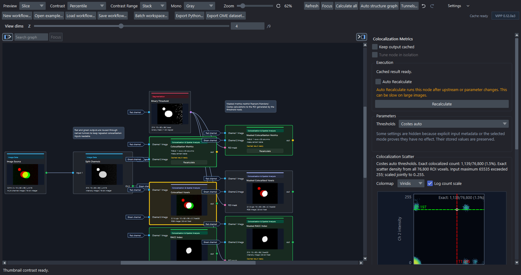
An undocked VIPP colocalization graph with parallel metrics and image branches and a scatter plot in the inspector

The same red/green channel outputs feed independent metric, voxel, and RACC branches. The selected calculated node exposes its threshold scatter for QC.

What The Scatter Inspector Calculates¶

The colocalization inspector calculates all three summaries over every voxel in the analysis population:

the total ROI population (or the complete image when no ROI is connected);
the number meeting both channel thresholds;
the complete two-dimensional scatter-density grid.

Large datasets are processed in bounded chunks and off the user-interface thread. Chunking limits temporary memory; it is not sampling. The density image, ROI count, and colocalized count all represent the complete ROI population. The detached scatter window supports up to 4,096 bins per axis with a host-memory preflight. The compact inspector uses a mass-preserving derivative of at most 1,024 bins per axis, not a sample of source voxels. Existing graph scatter nodes also support independently configured histogram bins and square output size.

For example, a summary such as Exact colocalized count: 18,420/251,006 means that all 251,006 ROI voxels contributed to both the count and the displayed density. The scatter grid is a visual QC summary; the metric table and Colocalized Voxels output remain the appropriate quantitative artifacts.

Dragging a threshold guide previews its position and an immediate density-derived count without invalidating the workflow on every movement. Releasing it commits the threshold, switches the node to manual thresholds, and recounts the complete ROI. This is a scientific parameter change, not merely a plot adjustment: wait for the exact count, recalculate stale manual outputs, and save the workflow afterward.

Use Open in window in the scatter section of Colocalization Metrics or its masked variant for a larger interactive view. Colormap and log-density changes redraw cached density; bin changes calculate a new density in the background. Export size controls square PNG or TIFF output independently of the window's size.

Both axes use a zero-inclusive shared range by default. Zoom to populated data uses the selected percentile range; Equal axis scales makes equal intensity differences occupy equal distances. The range readout identifies what is visible. These display choices never clip the population used for exact counts or metrics.

The old Colocalization Scatter Plot and masked graph nodes are hidden from the palette, but remain executable in saved workflows and headless programs that require their durable raster output. New interactive work should use the metrics-node pop-out.

Native intensity and metric names in 0.13 and later¶

Pearson no-threshold and threshold-domain outputs now expose canonical names that distinguish an any-channel-below-threshold (OR) population from the both-channels intersection. Shorter older column names remain aliases for compatible table consumers; use the canonical names in new reports.
Fiji Manders M1/M2 and thresholded tM1/tM2 are reported separately. Existing manders_m1 and manders_m2 columns now alias thresholded tM1/tM2. The older above-threshold intersection fractions remain under descriptive non-Manders names.
Automatic Costes thresholds target Fiji Coloc 2 3.1.0's classic search, including native one-unit steps and its population/tie behavior. This is a source-aligned compatibility implementation, not completed independent parity certification.

Pixel and object tables record coloc_semantics=fiji_coloc2_3.1 and coloc_validation_status=experimental_source_aligned_golden_parity_pending. Archive both fields and the exact column names used in analysis. Independent Fiji-generated golden parity remains pending, so validate this path externally before consequential use.

Object Colocalization¶

labels + channel 1 + channel 2
  -> Object Colocalization Metrics

This produces one row per object and is designed to merge with object morphology and intensity tables.

Label Association¶

Overlap between two object sets:

reference labels + target labels
  -> Label Overlap Association

Nearest centroid association:

reference labels + target labels
  -> Nearest Object Distance

Event or puncta assignment:

events / puncta + regions / ROIs
  -> Event Localization

Reference Workflows¶

Workflow	Purpose
`synthetic-colocalization-racc.json`	New in 0.15.0a5: focused whole-image and ROI-masked RACC-like index output, threshold review, method explanation and citation.
`synthetic-colocalization-overlap.json`	New in 0.15.0a5: whole-image and ROI-masked overlays/metrics, Boolean overlap masks, 3D cleanup and connected-region measurements.
`synthetic-object-colocalization-association.json`	Object colocalization rows, label overlap, nearest-object distance, event localization, and merged tables.

Reporting Checklist¶

For exact exported definitions, see Pearson, Manders, and Costes, the RACC-like index, and object-association fields.

Report:

channels analyzed;
preprocessing steps;
threshold mode and final thresholds;
analysis population: whole image, ROI, or object labels;
how the ROI was defined and its voxel count;
whether intensities were normalized or clipped;
native intensity units and the exact metric column names/semantic status;
scatter histogram bins, output size, clipping, and axis range when a scatter image is retained as evidence;
2D/3D and leading-axis handling;
ROI or label-generation method;
RACC parameters if using RACC-like outputs.

Validation Note¶

The current implementation has frozen method documentation and automated regression tests, but independent Fiji-generated numerical parity remains pending. Broad cross-tool or biological validity claims still require external comparisons, positive/negative controls, and assay-specific validation.