Tour a finished workflow
This tour uses a complete, tested graph. You will inspect it—not rebuild it—so you can learn the interface before dealing with graph editing.
Open the example
Choose:
New in 0.15.0a5: Select an example to read its purpose, Input data, short What to explore and What you'll get bullet lists, and a Try this suggestion. Each action or expected output is listed separately. Search by name or task to narrow the list, then click Open example (or press Enter) to open it in a new workflow tab. Cancel is to the left of Open example at the bottom of the chooser. Browsing the descriptions does not calculate anything. Compact margins leave more room for the list and description, which have contrasting backgrounds in both light and dark themes. Drag the divider to adjust their widths; in a narrow window, the description moves below the list.
The Image Source is set to VIPP synthetic multichannel volume. Its channels
are blue, green, and red; this workflow uses the red/TRITC-like channel.
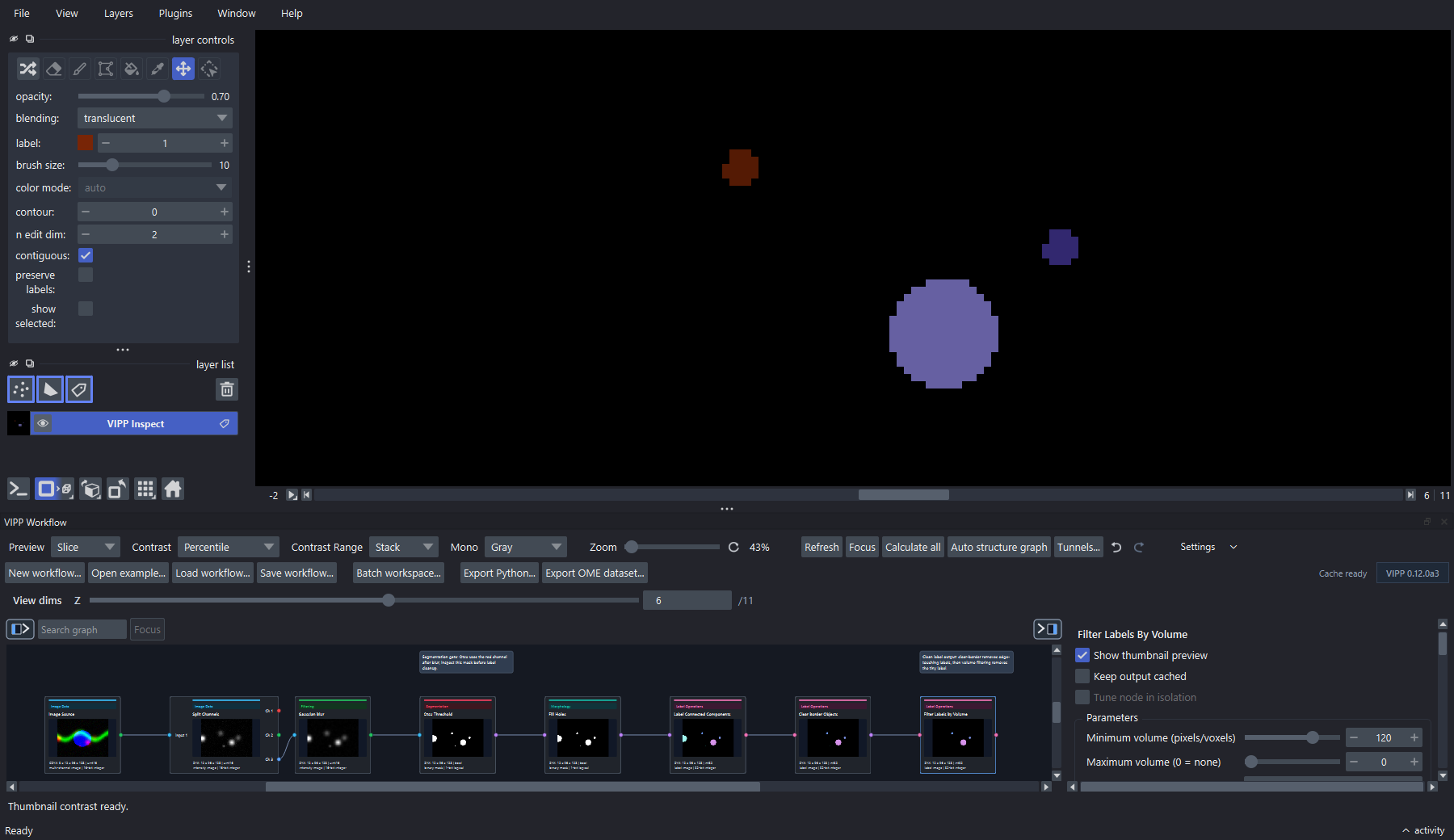
The overview was captured in 0.15.0a1; its Preview menu is named Display settings in 0.15.0a2. The demonstrated workflow remains the same.
Full interface context for the tour: the graph runs left to right below the napari viewer, and the selected volume filter is editable in the inspector.
Read the graph from source to result
flowchart LR
  A["Image Source"] --> B["Split Channels"]
  B --> C["Gaussian Blur"]
  C --> D["Otsu Threshold"]
  D --> E["Fill Holes"]
  E --> F["Label Connected Components"]
  F --> G["Clear Border Objects"]
  G --> H["Filter Labels By Volume"]
Each connection carries data from an output port to a compatible input port. The visible graph records processing order, but it does not contain cached pixel arrays.
Inspect one decision at a time
Select each node from left to right:
- Split Channels: confirm which output is the red signal.
- Gaussian Blur: compare the source and smoothed thumbnails.
- Otsu Threshold: inspect the binary foreground mask.
- Fill Holes: look for changed interiors, not only object outlines.
- Label Connected Components: confirm touching structures did not become implausible single objects.
- Clear Border Objects: confirm that edge-touching biology was intentionally excluded.
- Filter Labels By Volume: inspect the incoming size distribution and the labels that were removed.
New sessions request Auto compute. After each calculated node, read its compact CPU/GPU badge rather than assuming Auto used a GPU. Auto begins with reviewed safe GPU defaults. After accelerated-only exact compatible history, the next global Auto run measures CPU once on the same execution surface; a later matching run applies the 1.20x/20-ms gate. The exact data, environment, exploration step, or learned CPU result can therefore produce an ordinary CPU decision. This tour does not require GPU setup; use Prefer GPU or Custom with the CPU/GPU guide after you understand the graph and its outputs.
Use Pin selected to keep an important output as a napari layer while you select another node. A pinned layer is for comparison; it is not a new graph connection.
Change a parameter safely
Select Gaussian Blur, note its current value, and make a small change. Watch the threshold mask and final labels update downstream. Undo the edit with the toolbar undo action.
This demonstrates a central property of an interactive graph: one parameter can change every downstream result. The ability to see that change helps with review, but it does not tell you which value is biologically correct.
Recognize manual nodes
Measurement, graph-analysis, RACC, and deconvolution nodes can use a manual/cached calculation policy. When one is stale or has not run, select it and choose Calculate or use Calculate all. After upstream changes the button may read Recalculate.
Save a copy
Choose Save workflow and save the JSON under a new name. Reopen it with Open. The graph and settings should return; cached images and tables are deliberately recomputed from a source.