Object Measurements And Tables¶

Measurement workflows start from labels and produce tables.

Inspect and export the complete table¶

Select a calculated measurement node and expand Results. The compact table provides a quick preview; Open in window opens every row in a resizable result-table window. Click column headings to sort and inspect outliers, units, missing values, and per-object status/error fields.

Sorting is display-only. Export CSV/TSV… writes the exact scientific table in workflow row order, not the sorted presentation order. If upstream data or parameters changed, recalculate the stale manual result before exporting it. The result window shows the stale/current state rather than silently treating an old table as a new calculation.

Reproducible intensity histograms¶

Intensity Histogram produces a full-data table from one connected numeric array. Choose bin count, data-derived or custom bounds, and linear or logarithmic bin spacing. These are scientific settings saved with the workflow, unlike a display-only inspector histogram. The node is manual/cached by default.

Its table contains bin edges, centres, widths, counts, fractions, densities, and cumulative values. Non-finite values are excluded; custom-range underflow and overflow and values excluded from logarithmic bins are recorded in metadata. Review those counts instead of assuming every pixel fell inside the plot.

The inspector and histogram pop-out use the calculated table without rereading the source to redraw it. Switching between count, fraction, density, or cumulative views changes presentation, not the bin calculation. Use Results to inspect or export the exact values. A comparison between different images still needs an explicit shared range, common bin edges, and a justified normalization.

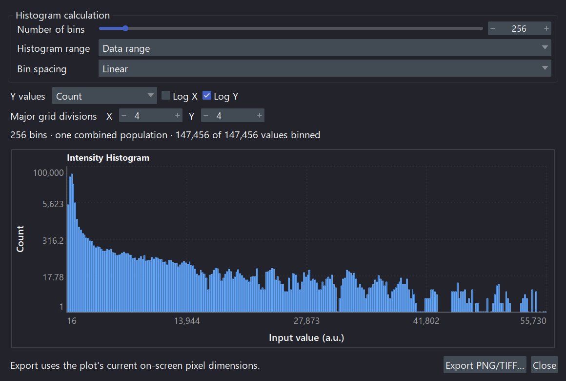
The detached intensity-histogram window showing a synthetic distribution with labelled plot and export controls

The histogram is a view of the cached scientific table. Retain its bin edges and excluded-value metadata when reporting the distribution.

Basic Object Measurement¶

labels
  -> Measure Objects

Measure Objects reports object identity, size, centroid, bounding box, equivalent diameter, extent, Euler number, and optional morphology groups. When spatial scale metadata exists, physical-unit columns are emitted where the calculation is well-defined.

Object Plus Intensity¶

labels + matching intensity image
  -> Measure Objects + Intensity

This produces object morphology plus per-label intensity summaries such as mean, minimum, maximum, sum, and standard deviation.

Use this when you want measurements such as:

intensity per nucleus;
reporter intensity per cell;
channel intensity inside segmented objects;
object features for PCA or treatment separation.

CPU and GPU measurement coverage¶

In 0.15.0a1, the CuPy candidates for label-table measurements cover only the basic Measure Objects and Measure Objects + Intensity schemas. They require native-endian, non-negative int32 labels in resolved 2D/3D leading blocks. The intensity variant additionally accepts matching Boolean, uint8, uint16, or finite float32 intensity data.

Enabling shape/axis/boundary descriptors, derived ratios, 2D moments, or other extended groups keeps the complete node on the authoritative CPU path. This is expected and appears in the node decision; the GPU provider never returns a reduced table while pretending the requested schema was complete. Its bounded device calculation is finished by an exact typed host-table finalizer that preserves schema, row/column order, units, integer fields, and missing-value semantics. A one-pixel object's population standard deviation is exactly zero.

The standard gpu-cuda13 extra includes these CuPy providers. No separate provider build or installation is required. See the Windows NVIDIA GPU guide and choose and verify compute.

VIPP 0.15.0a1 additionally provides a hybrid GPU path for Measure 3D Mesh Morphology on supported non-negative native int32 3D labels. The GPU packs label regions; marching cubes, convex hulls, and exact public table construction remain authoritative CPU work. A GPU badge therefore does not mean every part of a mesh calculation ran on the device or that it must be faster.

Analyze Skeleton has a reviewed CuPyX path for Boolean, already-skeletonized 2D/3D inputs. Requesting skeletonization first remains CPU work. Both providers retain dtype, shape, environment, memory, and scientific admission gates. See the compute matrix for scope.

3D Mesh Morphology¶

3D labels
  -> Measure 3D Mesh Morphology

Use this for true ZYX labels when surface area, mesh volume, sphericity, convex hull metrics, or 3D solidity matter.

This node is manual/cached because mesh calculations can be expensive.

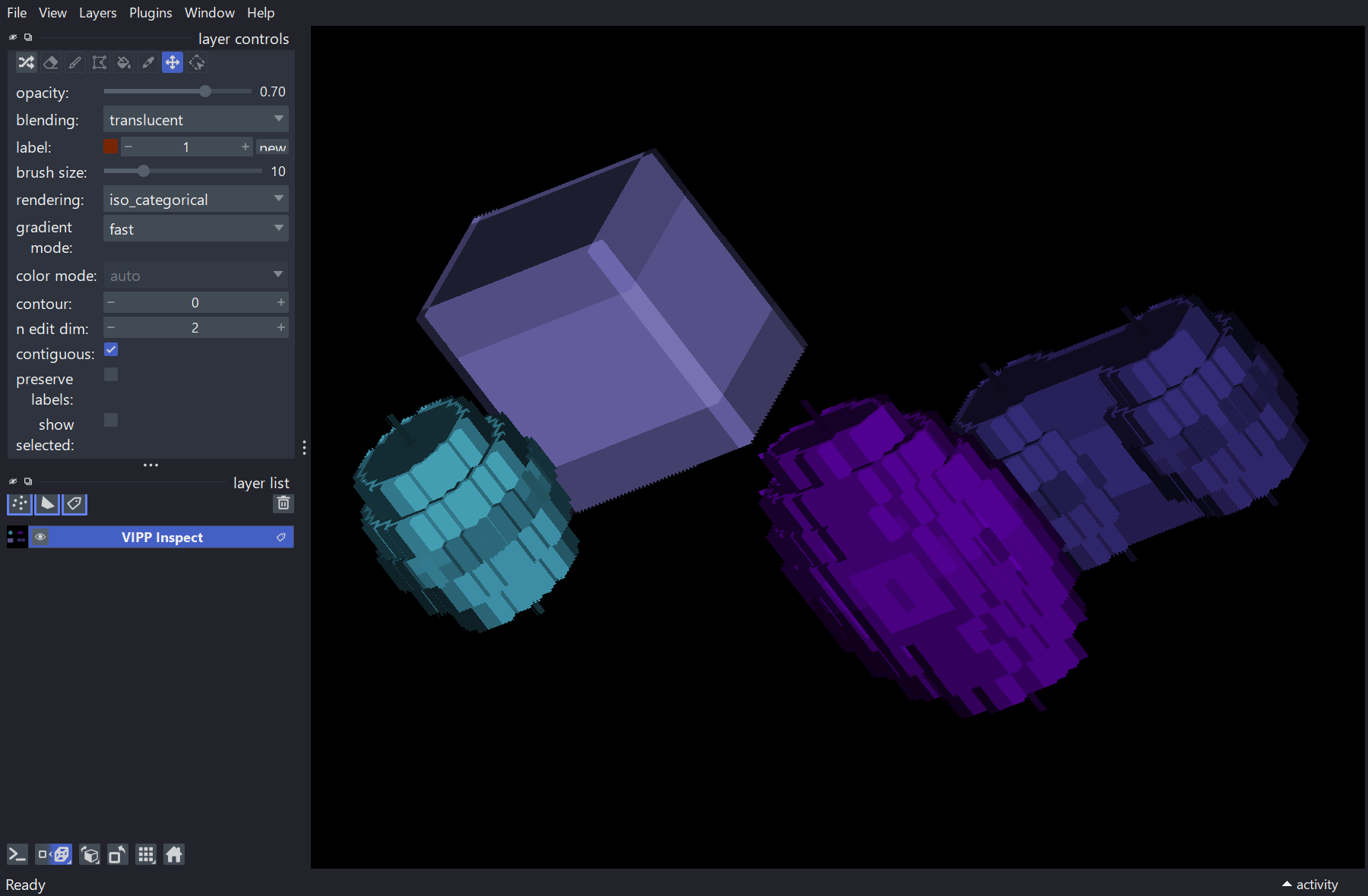
A napari 3D rendering of the synthetic anisotropic label objects used for mesh-morphology review

Inspect the 3D label geometry as well as the resulting table. The bundled phantom includes varied shapes and anisotropic calibration for regression and demonstration—not biological validation.

Table Assembly¶

Manual/cached sibling measurements can be calculated in either order. Since 0.14.0a1, re-reading or re-materializing the same unchanged file revision does not stale a ready sibling merely because Python created a different array wrapper. For example:

labels -> Measure Objects -----------------> Merge Tables
      \-> Measure 3D Mesh Morphology ------/

Calculate both manual nodes. Each should remain ready, and Merge Tables should become calculable once it has both coherent tables. This also applies when low-memory cache pruning re-materializes the same pinned source revision.

A genuine edit still invalidates the appropriate descendants. Recheck both branches after changing the source file/revision, labels, intensity input, parameters, or connections. If siblings alternate between ready and stale without any such change, preserve the workflow and execution details and report the problem; repeatedly recalculating is not a valid workaround for an incoherent merge.

flowchart LR
  L["Labels"] --> M["Measure Objects"]
  L --> I["Measure Objects + Intensity"]
  X["Matching intensity image"] --> I
  L --> D["Measure 3D Mesh Morphology"]
  M --> J["Merge Tables"]
  I --> J
  D --> J
  J --> S["Select Table Columns"]
  S --> A["Add Metadata Columns"]
  A --> U["Summarize or Batch Output"]

Only merge branches that share compatible identity keys and meaning. A table with the expected row count can still be wrong if time, label, or source identity columns were dropped or misaligned.

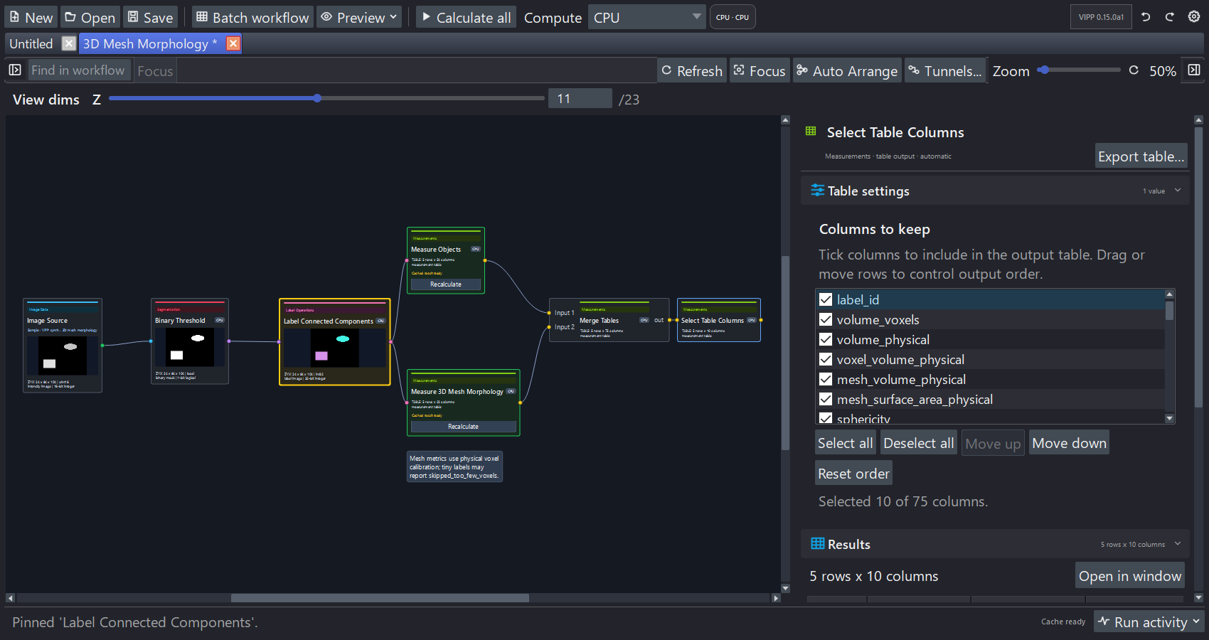
An undocked VIPP mesh-morphology workflow with calculated measurement branches and a selected ten-column table

The bundled mesh example combines calibrated object and mesh measurements, then selects a compact table whose rows, columns, units, and values can be reviewed before export.

Reference Workflows¶

Workflow	Purpose
`red-channel-object-intensity-measurements.json`	Labels plus matching intensity image into `Measure Objects + Intensity`.
`red-channel-merged-measurement-table.json`	Object morphology, intensity, table merge, and metadata columns.
`synthetic-measurement-summary.json`	Grouped summaries with known object counts and areas.
`synthetic-derived-object-morphology.json`	Derived 2D morphology, circularity, and Hu moments.
`synthetic-3d-mesh-morphology.json`	True-3D mesh morphology on anisotropic synthetic objects.

What To Check Before Export¶

Use measurement tables and units for identity keys, unit propagation, physical-column limits, and mesh-status fields.

Are labels correct?
Are label IDs stable after filtering?
Are scale and units correct?
Are leading axes such as time represented by identity columns?
Do table units match the reported measurement?
Have metadata columns such as treatment, replicate, or batch been added?