Inspect and compare outputs

VIPP has several inspection surfaces. Choose the one that answers the question rather than treating a thumbnail as evidence for every decision.

Surface	Good for	Not sufficient for
Node thumbnail	Rapid whole-graph scan	Fine boundaries, rare failures, or quantitative QC
Inspector preview	Selected node at a controlled slice/MIP	Comparing many full-resolution layers
Pinned napari layer	Full-resolution comparison and overlay	Recording why a parameter was selected
Histogram	Dynamic range and threshold context	Spatial correctness
Label-volume histogram	Size-filter cutoff review	Shape or identity correctness
Table preview	Columns, rows, units, obvious missingness	Statistical validation of measurements

Use the inspector for the selected data

The inspector now presents sections according to the node's scientific role. Image operations show intensity distributions; masks show foreground occupancy; labels show object-size distributions rather than a misleading histogram of label IDs. Filter Labels By Property shows the selected measurement and range. Metadata-only nodes emphasize axes and calibration without duplicating an unchanged intensity histogram.

Measurement nodes put Results near their settings. Colocalization nodes prioritize joint scatter and thresholds. Shared Behavior, Compute, Output Metadata, and history sections remain available below. Expand the section you need; the inspector is not a requirement to use every diagnostic.

Connected inputs identify which branch supplies each named input. When a node has multiple outputs, select the output you intend to inspect or save. Always check whether the displayed result is current, stale, or still calculating.

Read Display Summaries Correctly

An inspector histogram counts every finite value in the chosen slice or stack, then groups those counts into a compact chart. Its chart bins are independent of the saved Float histogram bins used by histogram-based automatic threshold nodes. Changing plot log scale or appearance does not change the mask.

The colocalization scatter density, ROI population, and colocalized count are also calculated over every ROI voxel. Threshold-independent density remains visible while exact threshold-dependent counts are recalculated, but a calculating count is not final evidence. The compact inspector uses a mass-preserving representation of at most 1,024 bins per axis; the detached scatter window can retain and render up to 4,096 bins per axis. On a large input, wait for the exact background calculation to finish before capturing a QC screenshot or recording a count.

Napari contrast limits are display-only. For a large inspect or pinned layer, VIPP may show an explicit provisional dtype range first and replace it with the exact full finite range when the background calculation completes. A manual contrast adjustment made while waiting is preserved. Neither range changes the node output or downstream measurements.

Tune Thumbnail Speed And Detail

Use Preview → Detail for the rendered image and Preview → Range for the statistics workload; they solve different problems.

Goal	Setting
Fast card redraws while editing	Low (90 × 55) detail.
Default balance	Standard (180 × 110) detail.
More backing detail for HiDPI display or downsampling	High (360 × 220) detail.
Maximum graph zoom still looks pixelated	Very High (720 × 440) detail.
Stable brightness across T/Z/C	Stack contrast; wait for its cached exact limits.
Avoid a full-output contrast scan	Slice contrast; it normalizes the selected detail's sampled current view.

The card viewport remains fixed, and High/Very High retain larger source images rather than guaranteeing a larger on-screen card. Very High uses four times the backing pixels of High, so reserve it for maximum zoom or dense displays. Detail can slightly change Slice limits because Slice normalizes the selected resolution's spatial sample. Low detail does not make Stack statistics cheaper: Stack remains full-output and resolution-independent, and Auto routes it from the full output dtype and byte size. Eligible uint8/uint16 Stack Percentile uses an exact histogram on CPU or CuPy; Min-max uses an exact native CPU reduction. Auto's conservative cold GPU crossover is 384 MiB for uint8 and 512 MiB for uint16, becoming 32 MiB after the histogram path is warm. These measured defaults are heuristics rather than universal fastest guarantees. Float and other-dtype percentiles remain on the exact NumPy-compatible CPU path.

Choose Settings > Thumbnail statistics > CPU to avoid CUDA initialization, or Prefer GPU to attempt every eligible CuPy histogram with visible CPU fallback. Main compute CPU always wins and forces statistics to CPU; main Prefer GPU biases thumbnail-statistics Auto toward GPU. Main Auto and Custom use adaptive presentation routing.

Select a node and read the compact Thumbnail contrast row near the top of its inspector—Calculating… / CPU · NumPy / GPU · CuPy / CPU fallback / Error—for presentation state. Hover that row or the thumbnail for algorithm, bytes, time, reason, threshold, fallback, or failure; keyboard What's This help and screen readers receive the same text. Do not confuse it with the scientific compute badge that remains in the node title row. While Stack statistics run, the shared toolbar shows the active node/backend/phase and Cancel keeps the provisional thumbnails without publishing partial limits. CPU integer work advances and cancels between bounded chunks. An active GPU kernel/synchronization or float/other-dtype NumPy percentile may have a non-interruptible inner pass; VIPP identifies the phase and cancels at the next cooperative boundary.

Recalculating the same selected node/output preserves its compatible display profile and the napari camera, displayed dimensions, slice positions, zoom, translation, and rotation. Switching to another output restores that output's own saved profile or safe defaults, so styles do not leak between scientific results. Use the inspector header's reset-to-defaults action when you want to discard the selected output's remembered presentation.

Pin an output in napari

1. Select a node with an image-like output.
2. If it has several outputs, select the intended output port.
3. Choose Pin selected.
4. Rename the napari layer if necessary so the operation and parameters remain recognizable.

Pin the raw image, a decisive intermediate mask, and the final labels for an overlay review. Hide or show layers to locate false positives, missed objects, merged objects, and boundary errors.

Verify what implementation produced the output

After an accepted calculation, read the card's compact CPU, GPU · CuPy, or amber CPU fallback badge. A muted badge belongs to the last accepted result while the node is stale or updating. Hover or inspect the node for the implementation ID/version, decision reason, memory estimate, and fallback details. The toolbar mode is only the request; it cannot establish what produced the displayed pixels or table.

See choose and verify CPU or GPU compute before comparing or benchmarking implementations.

Inspect colocalization scatter at useful resolution

Select Colocalization Metrics or its masked variant and use Open in window in the scatter section. The larger resizable view provides density bins, colormap, logarithmic density, populated-range zoom, equal-axis scales, and PNG or TIFF export at an explicit Export size.

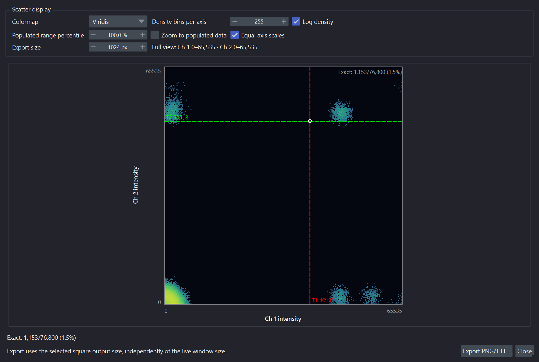
Display controls change the density picture. Moving and releasing a threshold guide changes a scientific parameter and requires a new exact count.

The default zero-inclusive shared axis range lets equal intensity differences have equal visual lengths. Zoom to populated data uses the chosen populated range percentile; Equal axis scales preserves equal intensity units per pixel. View bounds and density clipping change the picture, not the complete ROI used for exact counts and metric tables.

Colormap and log-density changes redraw retained data immediately. Re-binning runs in the background with a memory preflight. The pop-out supports up to 4,096 bins per axis; the smaller inspector uses a bounded mass-preserving derivative rather than sampling source voxels.

Dragging a threshold guide previews its position and a density-derived count. Releasing it commits the scientific threshold and requests the exact full-ROI count. Wait for that exact result before recording it. Plot display settings alone do not change the workflow's thresholds.

Legacy Colocalization Scatter Plot graph nodes remain executable in existing workflows and through headless calls when a durable raster is required, but are hidden from the palette. Use the metrics-node pop-out for new interactive scatter inspection.

Open a complete result table

In a table-producing node's Results section, use Open in window. This opens the complete table in a resizable sortable view, not only the compact inspector preview. Click a column heading to sort ascending, then again to sort descending. Review units, missing values, and status/error columns alongside the measurements.

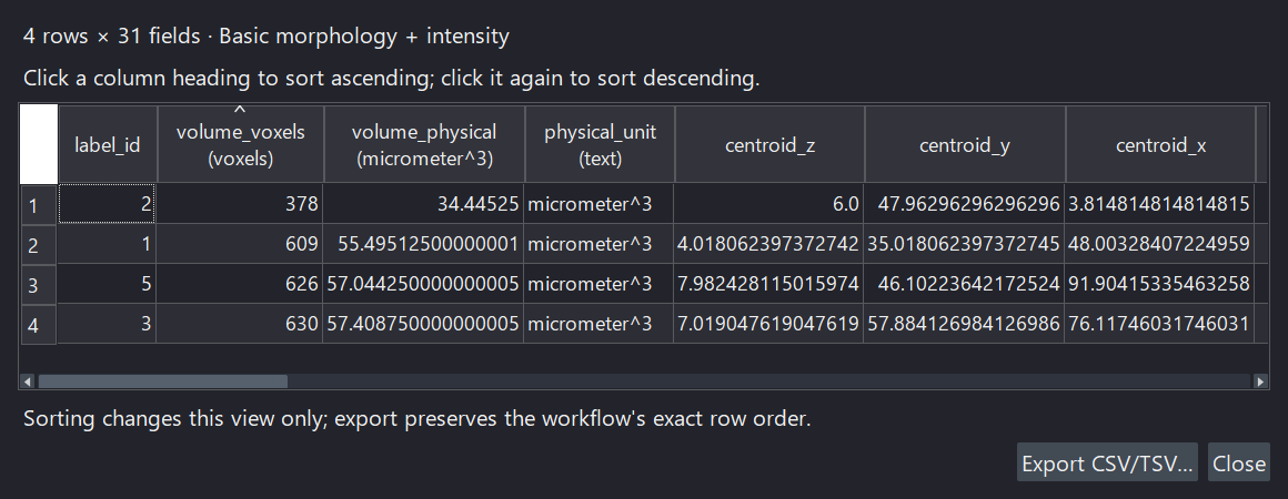
Open the full result when a compact preview is insufficient. Sorting affects only this view; export retains the workflow table's scientific row order.

Sorting changes the view only. Export CSV/TSV… preserves the workflow's exact row order. A result made stale by an upstream edit remains explicitly labelled; use Recalculate before treating it as a new result.

For a reproducible intensity distribution, add the manual Intensity Histogram node. Unlike a display-only histogram, its bin definition is part of the workflow and its full-resolution result is a table. See histogram and table workflows.

Compare 3D data without hiding failures

A maximum-intensity projection can make a workflow look persuasive while hiding slice-specific noise or z-merging. Review at least:

• representative YX slices at multiple z positions;
• the volume/MIP overview;
• objects near the top and bottom of the stack;
• regions with low signal or high background;
• anisotropic structures when z-spacing differs from x/y pixel size.

Use Link napari/VIPP sliders when synchronized slice navigation is useful. Turn it off when the inspector should remain on a fixed reference slice.

Review manual results after upstream changes

Manual/cached nodes become stale after a relevant upstream or parameter change. Select the node and choose Recalculate, or use Calculate all for all stale manual nodes. Do not take a screenshot or export a table while its status indicates a stale cached result.

Capture review evidence

For a formal analysis, retain representative QC images or screenshots with:

• input/sample identity;
• workflow and VIPP version;
• slice or projection mode;
• visible scale and units where relevant;
• enough context to identify the operation and parameter being reviewed.

Screenshots complement reference masks and quantitative tests; they are not a replacement for them.