Restore with a PSF

Born-Wolf PSF generation, measured-PSF preparation, Richardson–Lucy (RL), and RL with total-variation regularization (RL-TV) are public in 0.12.0a3. The deconvolution nodes are manual/cached so parameter changes do not repeatedly start expensive work without an explicit calculation. While a deconvolution is stale, its descendants wait and retain their last coherent cached results when those exist. A descendant with no prior output remains unavailable. Recalculating the deconvolution resumes that downstream branch.

Evidence boundary

Synthetic examples and automated checks support operation behavior. They do not establish broad restoration quality on real microscopes, acquisition settings, or biological targets. Review noise, ringing, edges, and apparent structures against an appropriate reference.

Read the PSF preflight

The RL and RL-TV inspector presents a read-only PSF preflight before expensive restoration. It groups evidence rather than rendering every diagnostic in the same warning color:

Status	Meaning	Response
Ready	All checks that can currently be performed passed.	Confirm that the PSF model and acquisition still match; Ready is not a biological-quality guarantee.
Warning	Calculation can run, but one or more conditions may reduce scientific reliability.	Read Needs attention and the corresponding What to do next actions before interpreting the result.
Invalid	A required property is incompatible or unsafe for the requested calculation.	Fix the invalid item before calculating.
Unknown	Inputs, values, or spatial rank are unresolved, or available metadata cannot be interpreted well enough to complete one or more checks.	Resolve or calculate the named input or repair its metadata, then return to the deconvolution node.

Missing physical calibration is a Warning, not Unknown: calculation can run, but VIPP cannot verify image-versus-PSF sampling compatibility and does not invent unit spacing.

Checks passed lists affirmative results such as compatible rank and physical sampling, finite non-negative values, normalization near one, odd dimensions, centering, contained support, or a met conventional-widefield Nyquist estimate. A passed item is not a warning simply because it contains numbers such as sum = 1 or peak offset = 0.

Needs attention separates warnings from invalid conditions and explains the specific consequence. Could not check identifies unavailable evidence rather than guessing. What to do next translates the detected issue into contextual actions; it does not silently modify, crop, resample, or normalize the scientific inputs.

The overall status is the most serious available result. A Nyquist warning is reported alongside PSF checks because it concerns acquisition sampling, while support and boundary-tail warnings concern the finite PSF and image arrays. These conditions can occur independently and can require different actions.

Use a measured PSF

The image and PSF are independent inputs; the two restoration methods branch in parallel for comparison:

flowchart LR
  I["Image Source"] --> RL["RL deconvolution"]
  I --> TV["RL-TV deconvolution"]
  P["PSF Image Source"] --> Q["Prepare / Validate PSF"]
  Q --> RL
  Q --> TV

1. Load the image and measured PSF in separate Image Source nodes.
2. Send the PSF through Prepare / Validate PSF.
3. Connect the same image and prepared PSF to each restoration branch.
4. Calculate one branch at a time while establishing safe parameters.
5. Compare each output with the unchanged input; do not feed RL into RL-TV when the intent is method comparison.

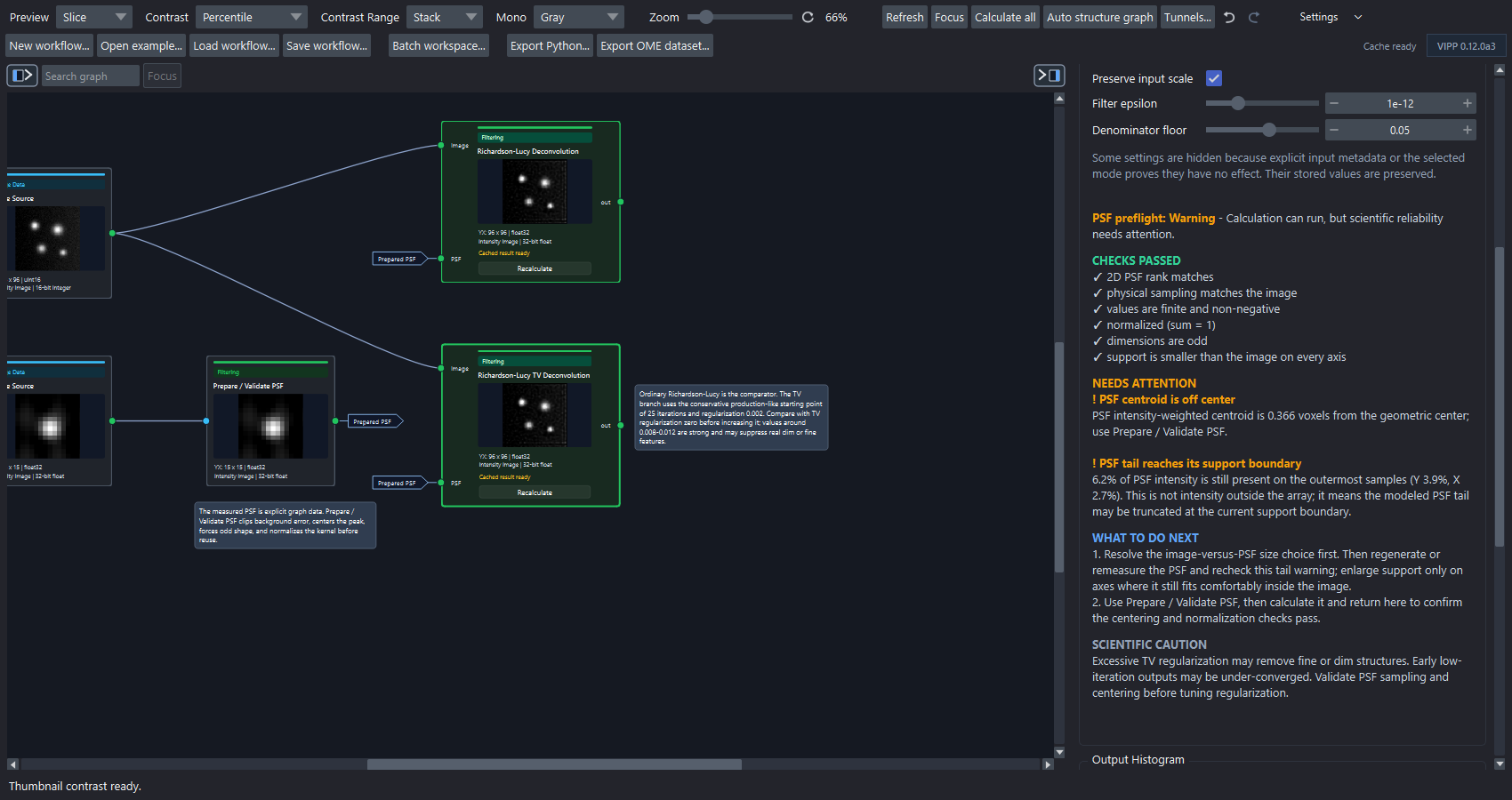
Both calculated alternatives use the same image and prepared PSF. The RL-TV inspector separates passed checks, attention items, and next actions instead of presenting every diagnostic as an undifferentiated warning.

Generate a Born-Wolf PSF

Born-Wolf PSF uses a reference image to resolve compatible axes/channels and can draw on supported pixel size, z-step, channel, and objective metadata. Explicit parameter overrides remain the user's responsibility.

flowchart LR
  I["Image Source"] --> B["Born-Wolf PSF"]
  I --> D["RL or RL-TV image input"]
  B --> Q["Prepare / Validate PSF"]
  Q --> D

Multi-channel reference data can produce dynamic PSF output ports. Inspect the resolved channel and dimensionality before connecting a restoration node.

Choose Born-Wolf support

The sampling interval, PSF support, and image extent are different quantities. Keeping them separate prevents several common configuration mistakes:

Quantity	Meaning	How VIPP obtains it
XY pixel size and Z step	Physical distance between neighboring PSF samples	Read from supported image metadata or entered manually
XY and Z support	Finite number of samples retained around the PSF center	Chosen by the user; the defaults are starting values
Image extent	Number of acquired pixels or planes available for restoration	Determined by the input image
Pupil samples	Numerical quadrature resolution for PSF generation	Chosen by the user; independent of spatial sampling and support

Auto from metadata can resolve physical sampling and supported optical parameters. It cannot determine one universally correct finite support. The ideal optical model has tails, so choosing an array boundary also chooses a truncation tolerance. VIPP keeps that choice explicit and checks the generated kernel rather than presenting a metadata-derived cutoff as exact.

The physical span shown beside a support field is the distance between the two outer sample centers:

physical span = (support samples - 1) x sampling interval

This value helps compare settings across datasets, but it is not by itself a pass/fail criterion.

A repeatable selection procedure

1. Resolve or enter wavelength, numerical aperture, refractive index, XY pixel size, and Z step. Confirm their units and channel assignment.
2. Review the widefield Nyquist result separately. A Nyquist warning describes acquisition sampling; increasing PSF support cannot reconstruct frequencies that were not sampled.
3. Begin with odd support dimensions. Calculate the Born-Wolf PSF.
4. Read the tail-containment result. VIPP measures the fraction of normalized intensity on the outermost one-sample shell. If it exceeds the current 1% practical threshold, increase the identified axis and calculate again.
5. Review image extent independently. The PSF should normally be smaller than the image on every processed spatial axis. If it is not, review boundary assumptions and whether the acquisition covers enough context.
6. Inspect the generated PSF and restored result. Check centering, normalization, ringing, edge behavior, noise amplification, and sensitivity to reasonable parameter changes.

What the tail percentage means

The percentage is intensity on the sampled boundary, not a measurement of intensity outside the array. Passing the check is a practical indication that the boundary values are small; it is not proof that all omitted tail energy is below exactly 1%.

Two warnings can therefore coexist without contradiction:

• Nyquist met, tail warning: the PSF is sampled finely enough, but the finite kernel window should be enlarged on the named axis.
• Tail check passed, image-extent warning: the kernel window contains its modeled tail adequately, but the image is too short on an axis for every output location to have complete support under the current boundary model.

The image-extent warning distinguishes equality from excess. When the PSF and image have the same number of samples on an axis, exactly one convolution alignment has full support and there is no surrounding fully supported interior margin. When the PSF has more samples than the image, no output position on that axis has full support. Both cases can calculate using the current zero-outside-image boundary assumption.

Do not shrink a PSF only to remove an image-extent warning. For volumetric restoration, possible responses include acquiring guard planes around the region of interest, interpreting or cropping affected output margins, or using 2D YX processing only when independent plane-wise imaging is the intended scientific model.

Why XY support is square

VIPP's scalar Born-Wolf generator uses one XY sampling interval and a rotationally symmetric optical model. It therefore produces a square YX kernel even when the camera frame is rectangular. The kernel describes the response around a point, not the camera field of view. A measured PSF or a more specific optical model is more appropriate when the system is astigmatic, spatially varying, or otherwise not rotationally symmetric.

Why some Fiji or ImageJ examples use image-sized PSFs

Software packages can impose different array-shape conventions while modeling the same physical sampling. The ImageJ deconvolution guide describes PSF width, height, and depth as PSF dimensions and permits a PSF equal to or smaller than the image. A PyImageJ 3D deconvolution example constructs an image-sized diffraction kernel for that particular operation.

VIPP accepts a smaller centered kernel, so its support dimensions do not need to equal the image dimensions. What must remain compatible is the physical sampling interval and spatial dimensionality. Matching the full image shape in VIPP can add substantial generation, memory, and convolution cost without improving the optical model.

Other user-set Born-Wolf parameters

Parameter	Practical interpretation
Pupil samples	Numerical integration accuracy. Use the default for ordinary work; for stringent validation, compare increasing values and stop when the generated PSF and downstream result have converged sufficiently for the analysis.
Normalize sum to 1	Normally keep enabled for Richardson-Lucy restoration so the PSF acts as a unit-sum blur kernel.
Channel	Confirm that the selected or automatically resolved wavelength belongs to the image channel being restored.
Spatial processing	Use 3D ZYX for a genuinely volumetric image and PSF model; use 2D YX only when planes are intended to be processed independently.

The Born-Wolf model and its Nyquist summary describe conventional widefield fluorescence. Reconstructed SIM, confocal, light-sheet, aberrated, or other modalities may require a measured or modality-specific PSF and sampling model.

Prepare and inspect the PSF

Depending on its settings, Prepare / Validate PSF can clip negative values, center the peak or centroid, normalize the sum, force odd shape, and reject an invalid kernel. Keep it visible in the graph so the actual kernel can be inspected independently from the restored image.

Check:

• dimensionality and sampling compatibility between image and PSF;
• centering and normalization;
• correct x/y pixel size and z-step;
• noise amplification, ringing, boundary artifacts, and invented-looking fine structure;
• sensitivity to iteration count and TV regularization;
• whether conclusions remain when compared with the original image.

Understand the RL-TV controls

Hover a Richardson-Lucy TV parameter label, slider, spinner, checkbox, or choice control for a concise effect-oriented tooltip. Slider ranges are practical exploration windows; the adjacent spinner is the exact-entry control and accepts valid values outside the slider window.

Parameter	Slider window	Interpretation
Spatial processing	Choice	Use 3D ZYX only for a true volumetric image/PSF pair; use 2D YX for independent planes.
Iterations	Linear 1–100	Start around 10–30. More iterations can recover detail but increase time and amplify noise, ringing, or PSF mismatch.
TV regularization	Geometric 1e-6–0.1	Larger values suppress noise more strongly but can flatten fine structure. Enter 0 in the spinner for ordinary RL behavior.
TV epsilon	Geometric 1e-12–1e-2	Smooths the TV gradient norm near zero; change it only with a defined stability test.
Filter epsilon	Geometric 1e-15–1e-3	Suppresses unstable ratio updates where predicted blur is tiny. Enter 0 in the spinner to disable it.
Denominator floor	Geometric 1e-3–1	Larger values limit extreme TV correction but can weaken the regularization update.

Normalize PSF is normally enabled. Clip negative input and Clip output negative are usually appropriate for non-negative microscopy intensity data, but clipping is a scientific choice. Preserve input scale maps the result back near the input intensity scale after internal normalization.

The positive logarithmic sliders use true geometric interpolation, making orders of magnitude accessible without sacrificing spinner precision. Do not treat the ends of a slider as validated parameter limits.

Bundled examples

Example	Purpose
deconvolution-2d	2D measured PSF with RL and RL-TV parallel branches.
deconvolution-3d	ZYX measured PSF and volumetric restoration branches.

Real bead-PSF and representative microscopy validation remains a high-priority evidence gap; see validation status.